Lesson 8: Monsters That Hide in Observational Studies

Lesson 8: Monsters that Hide in Observational Studies

Objective

You will learn about confounding factors that may impact the results of an observational study, which is why causation can never be concluded with observational studies, only associations between variables.

Materials

Computers
Spurious Correlations website: tylervigen.com

Vocabulary

cause, confounding factors, associated

Essential Concepts

Confounding factors/variables make it difficult to determine a cause-and-effect relation between two variables.

Lesson

In Lesson 6, you looked at the relationship between a student’s GPA and the number of friends that person has on social media. It seemed that students with higher GPAs had more friends than students with lower GPAs; but does did this mean that the cause of a person’s GPA is the amount of friends they have? NO!
You also identified other variables that could have contributed to the relationship. These outside variables are called confounding factors. Confounding factors are variables that are related to both the explanatory variable and the response variable in an observational study.
Ponder the statement below:

“Research suggests that a rise in umbrella sales leads to decreased crime rates.”

In your IDS Journal, write down possible confounding factors. You should choose a variable that is related to umbrella sales - one that might lead to decreased crime rates.
Now that you have thought of a few possibilities, study the following diagram progression to further understand the impact of confounding factors:
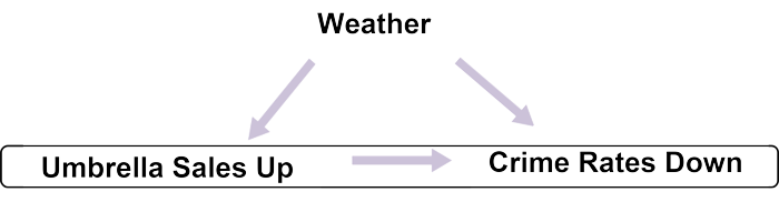
1. Step 1: The arrow shows that “a rise in umbrella sales leads to decreased crime rates”, since that is what researchers have stated.
2. Step 2: A variable that might be related to people buying more umbrellas - the confounding factor - might be the weather because, when it is rainy, people buy more umbrellas.
3. Step 3: You'll see an arrow going from “Weather” to “Crime Rates Down” because it is well known that when the weather is bad, people are less likely to be outside committing crimes.
4. Step 4: Remember that the original claim was that “a rise in umbrella sales leads to decreased crime rates”.” However, we’ve now shown that maybe buying umbrellas is not the only thing that could be contributing to a decrease in crime, which makes us question the link between the two variables.
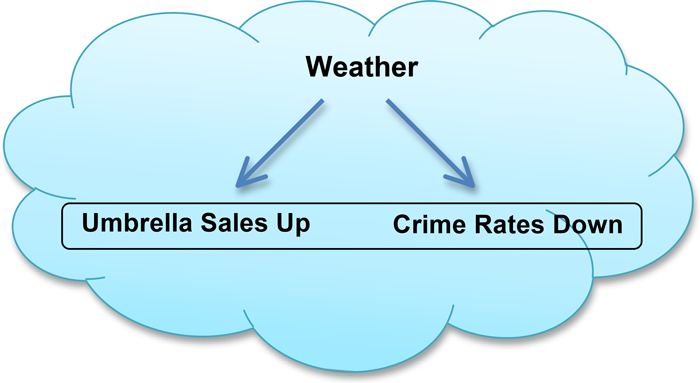
5. Step 5: Therefore, we have found a confounding factor with the variable “crime rates.” This means we can erase the original “link” between a rise in umbrella sales and decreased crime rates since there are outside variables interfering. We can’t say buying umbrellas causes decreased crime rates, but we can say that a rise in umbrella sales is associated with decreased crime rates.
Now that you have an understanding of what confounding factors are and how to identify them, take a look at the Spurious Correlations website by Tyler Vigen. This site shows many explanatory and response variables that are randomly associated with each other.
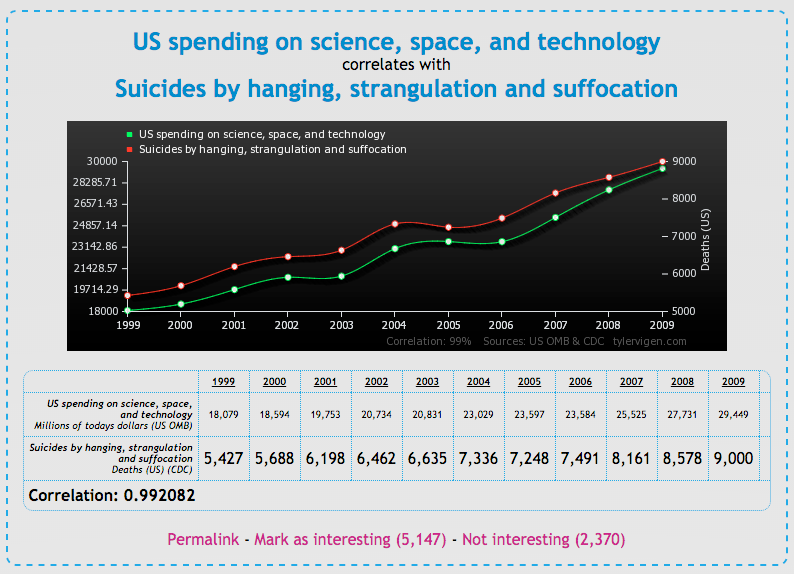
For the example given above, we see that as the U.S. spends more money on science, space, and technology, more people are dying by suicide. Clearly it does not make sense that if the U.S. keeps spending money on science, then more people are going to commit suicide. It simply happened by chance (or a bizarre chain of confounding factors) that the two variables are related to each other.
Explore the website on your own. Choose a graph that interests you and answer the questions below in your IDS Journal:

Note: There are multiple pages of graphs, so you are not restricted to simply the homepage. Also, this can be difficult, depending on the graph chosen. Some factors to consider: weather, economy, fashion trends.
1. What are the two variables shown in your graph?
2. Is there a positive association or a negative association between the variables?
3. Write an interpretation of this plot in the context of the data.
4. Write the data points in a "spreadsheet format" in a form that RStudio could read. Each row should represent a point on the graph, and each column one of the two variables.
5. By hand, make a scatterplot of the association. Describe whether the association seems strong, weak, or moderate to you.
6. Do you think that the explanatory variable causes the response variable? Explain.
7. If you answered "no" to f, then draw a diagram like in #4 with possible confounding factors.
Example answers to Step 7 are given below:
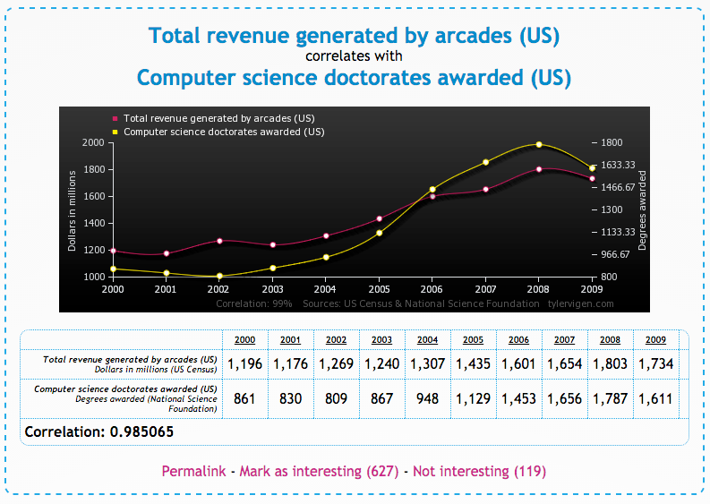
1. What are the two variables shown in your graph? Total revenue generated by arcades in the US and the number of computer science doctorates awarded.
2. Is there a positive association or a negative association between the variables? There is a direct relationship because the lines have the same shape (they follow the same pattern).
3. Write an interpretation of this plot in the context of the data. It seems that as more doctorates are awarded to computer scientists, arcades are generating more revenue.
  
  Arcade Revenue     CS doctorates
  
                      1196     861
  
                      1176     830
  
  etc.
4. Answers will vary.
5. Can you conclude that the one variable causes the other? No. Although the two variables are associated with one another, we do not have evidence to say that more doctorate awards cause arcades to make more money because the data do not come from a controlled experiment.
6. Draw a diagram like the one we did together earlier (in step 4 of lesson) with possible confounding factors. Student’s diagram should look like the one below:
Once you have selected a graph and have answered the above questions, share your responses with a partner. Explain why you thought your particular graph was interesting, how the two variables are related (directly or inversely), and whether or not there is a causal link between the variables.

Reflection

What are the essential learnings you are taking away from this lesson?

Next Day

LAB 3B: Confound it all!

Complete Lab 3B prior to Lesson 9.